The linear regression model is arguably the most widely used statistical and machine learning model. But what is it exactly? And how does it work?
Abstract
In statistics, the term linear model is used in different ways according to the context. The most common occurrence is in connection with regression models and the term is often taken as synonymous with linear regression model.
The General Linear Model
Linear regression models are used in everything from biological, behavioral, environmental and social sciences to business. Because linear regression is a long-established statistical procedure, the properties of linear regression models are well understood. This document aims at summarizing these properties.
The most straightforward case of a linear model is the simple linear regression model, where we only have one single dependent variable and a single independent variable . Note that we are denoting any scalars as small letters (), vectors as small bold letter (), and matrices as large bold letter (). Thus, we are dealing with one single coefficient in equation 13.1, and two vectors representing the data. Additionally, we take into account a , which is called the intercept. We can express multiple linear regression models (with one outcome variable and multiple predictors ) simply as: whereby is a vector with weights and is a vector with the error terms. The matrix product means, that we calculate the following for every observation : The intercept is a constant value that we add to every single prediction of the model. However, for the calculation, we simply add a constant column to the data. This makes it redundant to add it as a constant term in the matrix notation; but we need to remember to add a constant column to .
If we deal with multiple (correlated) independent variables, we might use the multivariate linear regression model. In that case, every part of the equation becomes a matrix. whereby is a matrix with the outcome variables, a matrix with the predictors (the design matrix), the matrix with the coefficients and is the matrix containing all error terms. The expression in equation 13.2 contains all linear models such as simple linear regression (Equation 13.1), multiple linear regression, multivariate regression (Equation 13.4), but also the (multivariate) Anova and Ancova. That is why it is also called the general linear model.
Different Loss Functions
For the following discussion, we assume that we are dealing with a multiple linear regression model as represented in equation 13.2. Therefore, we are dealing with a coefficient vector , a label vector and a design matrix .
In order to fit a hyperplane to our data, which is essentially what linear regression models do, we need to define what fitting well means. For that, we introduce the loss function . The task of finding the best fitting hyperplane now translates to the task of minimizing this loss function. One of the first loss function we could probably think of is to just minimize the distance of every prediction and the observation. This is called the absolute loss: Note that we have to take the absolute value of the difference between predicted and observed values (denoted with), because we want to punish any deviation from the models prediction, both positive as well as negative!
There is a dilemma, though: the absolute loss is not differentiable. Especially historically, this imposed a big problem: Being able to differentiate the loss function means that we can arrive at a analytical solution for the loss function, which is computationally very efficient. An alternative loss function which is differentiable is the squared loss.1 The squared loss is by far the most commonly used loss function for linear regression. However, one of its biggest downsides is that it’s very strongly influenced by the largest deviations from the model, so-called outliers. If we are dealing with too many outliers, we might consider to run a robust regression, which is less sensitive to deviations from any modelling assumptions. Consider for example the following loss function called the Huber loss: It resembles the squared loss within the tuning parameter ’s range and the absolute loss outside of it. This however imposes a immediate downside: we have to pick .
1 Besides the historical roots in computational efficiency, there are also other reasons for using the squared loss, discussed by the Gauss-Markov theorem.
Ordinary Least Squares
The most commonly used loss function for linear regression is the squared loss. We have seen before that this loss function comes with the nice advantage of an analytical solution to the minimisation problem; where we can calculate in one go (this is called the closed-form solution to the minimization problem).
In fact, this way of computing the coefficients is so common that we call it the ordinary least squares (OLS) method. The Gauss-Markov theorem states that the states that the ordinary least squares predictors are the best linear unbiased estimators (BLUE) for if the errors in the linear regression model are:
uncorrelated (),
have equal variances (),
and expectation value of zero ().
This means, that if the data generating function — which is responsible for the data we are seeing — is indeed linear, and its error follows the three Gauss–Markov assumptions, the ordinary least squares estimator will have no bias and the lowest possible variance. For Gaussian errors, the OLS estimator is equal with the maximum likelihood estimation, which we get by maximizing the likelihood function. In this case, denotes the th row of the matrix . However, according to the Gauss-Markov theorem, we do not need to assume this Gaussian distribution of the errors and will still end up with the maximum-likelihood estimates if the Gauss-Markov assumptions hold true!
This figure shows an example of the Gauss-Markov assumptions being valid (left), violated due to heteroskedasticity (center) and violated due to autocorrelation (right). The latter can be detected using (parital) autocorrelation functions.
However, even though Gauss-Markov theorem does not make any assumption about the distribution of the error term and we can have best unbiased estimates for the coefficients , we often also look at the statistical results (especially when we call the lm function in R), especially the p-values. Those are not per se a part of ordinary least squares, and they do very much assume that the errors are normally distributed!
Goodness of Fit
One of our core interest when looking at a model is its goodness of fit: how well does our model fit the underlying data. Or, on controversially, how much variance in the data is left unexplained by the model?
The difference between our model’s predictions and the observed values are called the residuals . Note how the coefficient vector is marked as the estimated coefficient vector . The residuals refer to the deviations of the data from our model. This is the core difference between them and the error term , which is the deviation from the true function: Closely related to the residuals, there are three metrics often calculated with a regression analysis: The sum of squared residuals (), the regression sum of squares (), and the total sum of squares ().2 Another value that can be computed for every linear regression model is the residual standard error (RSE). It is essentially an estimate of the standard deviation of the residual . The RSE is derived from the sum of squared residuals, and it becomes larger for (unnecessarily) added degrees of freedom. All these previously defined values give an idea of the model goodness of fit but they are hard to interpret because their unit depends on the particular model. Much easier to interpret is the coefficient of determination, which is the squared Pearson’s correlation coefficient between the predicted values and the observed values and thus lies always between 0 and 1. This metric can only increase with increasing number of predictors, and also for completely random input variables, it will approach 1 as approaches . Thus, it is not the best metric for the goodness of fit of a linear model!3 If anything, we should rather look at the adjusted R2.
2 Actually, the equation does not hold true in every instance of linear regression model — it assumes that the error follow a Gaussian distribution.
3 Except if tested on independent data, as it is often done following a machine-learning paradigm. However, in the classical use of linear regression we are often dealing with limited data sets, so this approach might not always be feasible.
Test Statistics for OLS
Normally, two tests are applied to a linear model: an F-test and a t-test. The F-test looks at the model as a whole, while the t-test evaluates the individual coefficients. The F-test assesses multiple coefficients simultaneously and give the p-value of the model overall. It can be used to compare different models (although only with the samy ). We can compute the F-score as follows: We can compute the p-value of the F-score by comparing it to the F-distribution, using the R function pf. The F-distribution is dependent on two degrees of freedom; and .
The test that we are probably most interested in is the t-test. The test is based on the assumption, that the errors are normally distributed. Based on this assumption, we calculate the probability of having estimated a coefficient as large or larger as we did under the unknown but true scenario of the null hypothesis .4 where are the standard errors of the predictors. The null hypotheses is that any predictor is zero; so that whole part can be dropped. We can compute the standard errors in the following way from the data and the residuals directly.5 where are the residuals, is the number of observations (number of rows in ) and the number of parameters (number of columns in ).
4 Note that the t-test does not return probability estimates of the coefficients themselves, which is a common misconception! To do this, we would need to use Bayesian inference.
5 However, R calculates the standard error via inverting the QR decomposition of the design matrix for processing speed reasons
The t-distribution is defined as follows: where is the gamma function and the degrees of freedom.
Given that, we can compute the p-value from the t-distribution using the pt function in R. Formally, the p-value is defined as: The direction from which we look at the t-distribution varies depending on the sign of the coefficient. To remedy that fact, we look at the absolute value of our t-statistic ().
As discussed above, the p-value is effectively the probability of getting a equal or more extreme estimation of a coefficient as we did when we assume the data generating function is a Gaussian with its mean being the null hypothesis and its variance being the variance of the residuals. Since we use the residual variance, the results of the t-test depends on the overall model specification. This is why specifying a model with different co-variables leads to varying p-values and significance levels for the same variable.
Weighted Least Squares
In our list of standard assumptions about the error term in this linear multiple regression model, we include one that incorporates both homoskedasticity and the absence of autocorrelation. That is, the individual values of the errors are assumed to be generated by a random process whose variance is constant, and all possible distinct pairs of these values are uncorrelated. This implies that the full error vector, , has a diagonal covariance matrix, .6
6 For some reason, the error covariance matrix is sometimes referred to as . Here, we use though because this is the standard way of denoting (any) covariance matrices.
To assess whether we should apply weighted least squares, we perform a Breusch-Pagan test.
After an initial OLS step, we can perform weighted least squares as follows: We calculate the weights by trying to predict the model’s residuals given the predicted values with a second OLS estimation.
-> Apply when the covariance matrix of the errors is not a diagonal matrix, but not a scaled version of the identity matrix.
We can estimate the covariance matrix of the residuals as follows:
Generalized Least Squares
-> Apply when the covariance matrix of the errors is not a diagonal matrix.
Non-spherical errors…
Linear Mixed Effects Models
A mixed model, mixed-effects model or mixed error-component model is a statistical model containing both fixed effects and random effects. In matrix notation a linear mixed model can be represented as follows. In this notation, is a known vector of obervations, where . Unlike in the OLS model, the errors of this mixed effects model are derived from two sources: on one hand from the error vector , but on the other hand also from the random effects , where we have both and . So, generally, the expected error in the model is still zero. However, by use of the term , errors might be clustered into groups, where is a design matrix containing information about these groups.
Estimation
This is how the linear mixed effects model is estimated according to Henderson (1954) (Henderson et al. 1959).
The linear model is fundamentally used for regression analyses. Formally, we can define a (multivariate) regression model as a function as follows. We call it a regression model whenever the response variable(s) is continuous. The predictors might be continuous, binary, nominal or ordinal. If was non-continuous, we would speak of (multi-class) classification and not regression.
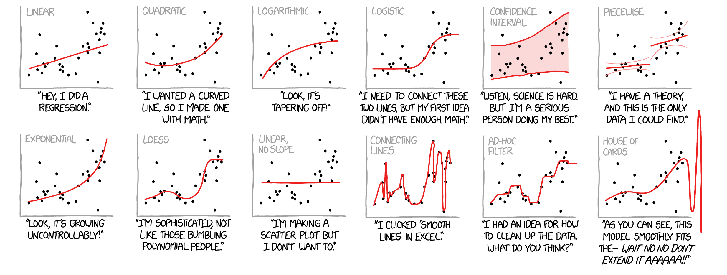
There are a lot of regression models
Curve fitting methods and the messages they send. Illustration by Todd Gureckis.
House of Cards is not a real method, but a common consequence of mis-application of polynomial regression — the model becomes extremely unstable at its fringes.
What linear models are used for
Inference: Establish whether a relationship exists – this combines the linear model with statistical tests.
Descriptive statistics: Develop an appropriate model to describe data which cannot be fully visualized anymore due to its dimensionality.
Prediction or Forecasting: Linear models are used to predict or forecast future values based on existing data. This could be anything from predicting future sales based on past data to forecasting weather patterns.
Functional form
Linear models describe a continuous response variable as a function of one or more predictor variables .
We may write this more compactly in linear algebra notation.
and are known, while and are unknown.
Components
Design matrix
A matrix containing the independent variable values a.k.a. the predictors a.k.a. the features.
Response vector
A vector containing the dependent variable values a.k.a. the response a.k.a. the labels.
Coefficient vector
A vector containing the parameters of the linear model — which are called the coefficients.
Error vector
A vector containing the errors of the model.
Finding the parameters
Loss minimization
The coefficient vector could theoretically have any form. However, we deem some of them better than others – we want to minimize the value of the residual .
We take the Euclidean norm () of the error vector , which means we calculate the loss () as:
Sum of squared error
Solving the equation
Extremely easy steps
Starting out with the equation for the LM, we want to isolate . We want to separate and . We know that , but only square matrices can be inverted. So, we multiply by .
This allows us quickly finding the solution for .
Model statistics
Two statistical tests are commonly applied
F-test: This test essentially compares two models. One model that includes the predictors of interest () and another reduced model that excludes these predictors ().
t-test: This test is used to determine if a single predictor variable has a statistically significant relationship with the response variable (, and ).
The F-test
In the linear regression model, we can calculate the -statistic as follows.
Here, refers to the degree of freedom of the error, while refers to the degree of freedom of the model. are the sum of squares of the model, and are the sum of squares of the errors.
The t-test
It’s all the same
How to apply this in R
Now that we know that , we can get the coefficients of any linear model using matrix multiplication (%*%) and transposition (t()).
y <- swiss$FertilityX <-cbind(Intercept =1, Agriculture = swiss$Agriculture)beta <-solve(t(X) %*% X) %*%t(X) %*% y
We can do this even faster with the lm() function.
model <-lm(Fertility ~ Agriculture, data = swiss)coefficients(model)
(Intercept) Agriculture
 60.3043752   0.1942017
Extensions
Mixed effects models
Polynomial regression
Regularization
Linearisation
Polynomial regression
Interactions
Weighted Least Squares
Weighted least squares (WLS) is a generalization of ordinary least squares (OLS) that can be particularly useful in several scenarios:
Heteroskedasticity: If the error terms in a regression model have non-constant variance across observations, it can lead to inefficient OLS estimates. WLS allows for the modeling of this non-constant variance by assigning weights that are inversely proportional to the variance of the error terms.
Incorporating Different Levels of Precision: In some datasets, different observations may be measured with varying degrees of precision. WLS can be used to give more weight to the observations that are measured with higher precision, reflecting the additional information they contain.
Modeling Correlation between Observations: If observations are correlated (as in time series or panel data), WLS can be used to model this correlation, leading to more efficient estimates.
Analyzing Survey Data: Often in survey data, different respondents or groups might be oversampled to ensure that the sample is representative. WLS can be used to weight the observations in a way that reflects the sampling strategy, ensuring that the estimates are representative of the population of interest.
Combining Information from Different Sources: If you are combining data from different sources that are measured on different scales or have different units, WLS can be used to appropriately weight the information from each source.
Fitting Models to Non-Linear Relationships: When fitting a linear regression model to a relationship that is inherently nonlinear, transforming the dependent and/or independent variables might create heteroskedasticity in the errors. WLS can be used to model this heteroskedasticity.
Robust Estimation: WLS can also be part of an iterative procedure to achieve robust estimates of regression parameters, by assigning lower weights to potential outliers or observations that have high leverage.
Generalized Estimating Equations (GEE): In longitudinal data, WLS is used as a part of GEE to account for the within-subject correlation, providing a more flexible correlation structure.
Weighted Least Squares is a versatile technique that can be applied in many different contexts to achieve more efficient, consistent, or representative estimates. It requires careful selection and justification of the weighting scheme, as an incorrect choice can lead to biased or inefficient estimates. The weights often need to be known (or estimated) up to a multiplicative constant, which means that it’s the relative weights that typically matter, not their absolute values.
Iteratively reweighted least squares
We can use iterative weighting for finding the coefficients of a model where a closed-form solution doesn’t exist. For example, we can apply the absolute loss function to a linear model, i.e. finding that satisfy: To find such a , we can run the following algorithm:
Estimate via OLS.
Calculate the weights as , where is the desired degree of the norm, i.e. in this case.
Estimate via weighted least squares using the weights from before.
Go back to step 2, using . Repeat until convergence.
p <-1B <-matrix(NA, nrow =500, ncol =ncol(X))model <-lm(Fertility ~ ., swiss)B[1,] <-coefficients(model)for (i in2:nrow(B)) { w <-abs(residuals(model))^{(p-2)/2} model <-lm(Fertility ~ ., swiss, weights = w) B[i,] <-coefficients(model)}
Generalized least squares
Generalized least squares (GLS) is a method used to estimate the unknown parameters in a linear regression model when there is a certain degree of correlation between the residuals in the regression model.
OLS: , i.e. the observations are uncorrelated, the covariance matrix of the errors is diagonal and a scaled identity matrix . OLS is useful if the Gauss-Markov assumptions are satisfied.
WLS: The covariance matrix of the errors is diagonal, but the variance is not constant. WLS is useful in the presence of heteroskedasticity.
GLS: is not diagonal, i.e. the errors are correlated. GLS is useful in the presence of autocorrelation.
Figure 13.1: Example of relationships where the Gauss-Markov assumptions are fulfilled (left), heteroskedasticity is present (center), and autocorrelation is present (right).
Linear Mixed Effects Models
A mixed model, mixed-effects model or mixed error-component model is a statistical model containing both fixed effects and random effects. In matrix notation a linear mixed model can be represented as follows. In this notation, is a known vector of obervations, where . Unlike in the OLS model, the errors of this mixed effects model are derived from two sources: on one hand from the error vector , but on the other hand also from the random effects , where we have both and . So, generally, the expected error in the model is still zero. However, by use of the term , errors might be clustered into groups, where is a design matrix containing information about these groups.
Estimation
This is how the linear mixed effects model is estimated according to Henderson (1954).
Regularization
Shrinkage estimator
Variable selection
Small n, large p problem
Henderson, C. R., O. Kempthorne, S. R. Searle, and C. Von Krosigk. 1959. The estimation of environmental and genetic trends from records subject to culling. Biometrics 15:192–218.
Source Code
---title: The Linear Regression Modelsubtitle: The linear regression model is arguably the most widely used statistical and machine learning model. But what is it exactly? And how does it work?abstract: In statistics, the term linear model is used in different ways according to the context. The most common occurrence is in connection with regression models and the term is often taken as synonymous with linear regression model.---## The General Linear ModelLinear regression models are used in everything from biological, behavioral, environmental and social sciences to business. Because linear regression is a long-established statistical procedure, the properties of linear regression models are well understood. This document aims at summarizing these properties.The most straightforward case of a linear model is the simple linear regression model, where we only have one single dependent variable $\mathbf y \in \mathbb R^n$ and a single independent variable $\mathbf x \in \mathbb R^n$.$$\mathbf y = \beta_0 + \beta_1 \mathbf x + \varepsilon$${#eq-SLR}Note that we are denoting any scalars as small letters ($a$), vectors as small bold letter ($\mathbf a$), and matrices as large bold letter ($\mathbf A$). Thus, we are dealing with one single coefficient $\beta_1$ in [equation @eq-SLR], and two vectors representing the data. Additionally, we take into account a $\beta_0$, which is called the intercept. We can express multiple linear regression models (with one outcome variable $\mathbf y \in \mathbb R^n$ and multiple predictors $\mathbf{X} \in \mathbb R^{n\times p}$) simply as:$$\mathbf y = \mathbf X \boldsymbol \beta + \boldsymbol \varepsilon$${#eq-MLR}whereby $\boldsymbol \beta \in \mathbb R^p$ is a vector with weights and $\boldsymbol \varepsilon \in \mathbb R^n$ is a vector with the error terms. The matrix product $\mathbf X \boldsymbol \beta$ means, that we calculate the following for every observation $y_i$:$$y_i = \beta_0 + \sum_{j=1}^p \beta_j x_{i,j} + \varepsilon_i$${#eq-MLR_written_out}The intercept $\beta_0$ is a constant value that we add to every single prediction of the model. However, for the calculation, we simply add a constant column to the data. This makes it redundant to add it as a constant term in the matrix notation; but we need to remember to add a constant column to $\mathbf X$.If we deal with multiple (correlated) independent variables, we might use the multivariate linear regression model. In that case, every part of the equation becomes a matrix.$$\mathbf{Y} = \mathbf{XB}+\mathbf{E}$${#eq-MVLR}whereby $\mathbf{Y} \in \mathbb R^{n\times l}$ is a matrix with the outcome variables, $\mathbf{X} \in \mathbb R^{n\times p}$ a matrix with the predictors (the design matrix), $\mathbf{B} \in \mathbb R^{n\times l}$ the matrix with the coefficients and $\mathbf{E} \in \mathbb R^{n\times l}$ is the matrix containing all error terms. The expression in [equation @eq-MLR] contains all linear models such as simple linear regression (@eq-SLR), multiple linear regression, multivariate regression (@eq-MVLR), but also the (multivariate) [Anova]{.smallcaps} and [Ancova]{.smallcaps}. That is why it is also called the general linear model.## Different Loss FunctionsFor the following discussion, we assume that we are dealing with a multiple linear regression model as represented in [equation @eq-MLR]. Therefore, we are dealing with a coefficient vector $\boldsymbol{\beta}$, a label vector $\mathbf y$ and a design matrix $\mathbf X$.In order to fit a hyperplane to our data, which is essentially what linear regression models do, we need to define what *fitting well* means. For that, we introduce the loss function $\mathcal L$.$$\boldsymbol{\hat \beta} = \arg \min_{\boldsymbol\beta} \mathcal L(\boldsymbol \beta)$${#eq-loss}The task of finding the best fitting hyperplane now translates to the task of minimizing this loss function. One of the first loss function we could probably think of is to just minimize the distance of every prediction and the observation. This is called the absolute loss:$$\mathcal L(\boldsymbol \beta) = \| \mathbf y - \mathbf X \boldsymbol \beta \|_1 = \sum_{i=1}^n \left| y_i - \hat y_i \right|$${#eq-absoluteloss}Note that we have to take the absolute value of the difference between predicted and observed values (denoted with$\|.\|_1$), because we want to punish any deviation from the models prediction, both positive as well as negative!There is a dilemma, though: the absolute loss is not differentiable. Especially historically, this imposed a big problem: Being able to differentiate the loss function $\mathcal L(\boldsymbol \beta)$ means that we can arrive at a analytical solution for the loss function, which is computationally very efficient. An alternative loss function which is differentiable is the squared loss.^[Besides the historical roots in computational efficiency, there are also other reasons for using the squared loss, discussed by the Gauss-Markov theorem.]$$\mathcal L(\boldsymbol \beta) = \| \mathbf y - \mathbf X \boldsymbol \beta \|^2 = \sum_{i=1}^n \left( y_i - \hat y_i \right)^2$${#eq-squareloss}The squared loss is by far the most commonly used loss function for linear regression. However, one of its biggest downsides is that it's very strongly influenced by the largest deviations from the model, so-called outliers. If we are dealing with too many outliers, we might consider to run a robust regression, which is less sensitive to deviations from any modelling assumptions. Consider for example the following loss function called the Huber loss:$$\mathcal L(y_i-\hat y_i) = \begin{cases} \frac{1}{2} \left( y_i-\hat y_i \right)^2 & \text{for } \| y_i-\hat y_i \| \leq \delta \text ,\\ \delta \left(\| y_i-\hat y_i \| - \frac{1}{2} \delta \right) & \text{otherwise.} \end{cases}$${#eq-huberloss}It resembles the squared loss within the tuning parameter $\delta$'s range and the absolute loss outside of it. This however imposes a immediate downside: we have to pick $\delta$.## Ordinary Least SquaresThe most commonly used loss function for linear regression is the squared loss. We have seen before that this loss function comes with the nice advantage of an analytical solution to the minimisation problem; where we can calculate $\boldsymbol \beta$ in one go (this is called the closed-form solution to the minimization problem).$$\boldsymbol{\hat \beta} = \arg \min_{\boldsymbol\beta} \mathbf \| y - \mathbf X \boldsymbol \beta \|^2_2 = \left( \mathbf X^\top \mathbf X \right)^{-1} \mathbf X^\top \mathbf y$${#eq-OLS}$$\begin{multlined}\mathcal L = \| \mathbf r \|_2^2 = \mathbf r^\top\mathbf r = (\mathbf y - \mathbf X \boldsymbol \beta)^\top(\mathbf y - \mathbf X \boldsymbol \beta) \\= \mathbf y \top \mathbf y - \mathbf y\top\mathbf X \boldsymbol \beta - \mathbf X\top\boldsymbol \beta \top\mathbf y + \boldsymbol \beta \top\mathbf X\top\mathbf X \boldsymbol \beta b \\\frac{\partial\mathcal L}{\partial \boldsymbol \beta} = \frac{\partial \left( \mathbf y^\top\mathbf y - \mathbf y^\top \mathbf X \boldsymbol \beta- \mathbf X^\top \boldsymbol\beta^\top \mathbf y + \boldsymbol \beta \top \mathbf X ^\top \mathbf X\boldsymbol \beta \right)}{\partial\boldsymbol\beta} \\= - 2 \mathbf y^\top\mathbf X +2 \mathbf X ^\top \mathbf X \boldsymbol \beta = \mathbf 0 \\2 \mathbf X^\top \mathbf X \boldsymbol \beta = 2 \mathbf y^\top \mathbf X \\\boldsymbol \beta = \left(\mathbf X ^\top \mathbf X \right)^{-1} \mathbf y^\top \mathbf X\end{multlined}$$In fact, this way of computing the coefficients $\boldsymbol \beta$ is so common that we call it the ordinary least squares (OLS) method.The Gauss-Markov theorem states that the states that the ordinary least squares predictors are the best linear unbiased estimators (BLUE) for $\boldsymbol \beta$ if the errors $\varepsilon$ in the linear regression model are:1. uncorrelated ($\text{Cov}(\varepsilon_i,\varepsilon_j) = 0, \; \forall \; i\neq j$),2. have equal variances ($\text{Var}(\varepsilon_i) = \sigma^2$),3. and expectation value of zero ($\mathbb E(\varepsilon_i)=0$).This means, that if the data generating function --- which is responsible for the data we are seeing --- is indeed linear, and its error follows the three Gauss–Markov assumptions, the ordinary least squares estimator will have no bias and the lowest possible variance. For Gaussian errors, the OLS estimator is equal with the maximum likelihood estimation, which we get by maximizing the likelihood function.$$\max_{\boldsymbol \beta} \left\{\prod_{i=1}^n \frac{1}{\sigma_{\mathbf y} \sqrt{2\pi}}\exp \left[ -\frac{1}{2} \left( \frac{y_i - \boldsymbol \beta^\top \mathbf x_i}{\sigma_{\mathbf y}}\right)^2 \right] \right\}$${#eq-likelihood}In this case, $\mathbf x_i$ denotes the $i$^th^ row of the matrix $\mathbf X$. However, according to the Gauss-Markov theorem, we do not need to assume this Gaussian distribution of the errors $\boldsymbol \varepsilon$ and will still end up with the maximum-likelihood estimates if the Gauss-Markov assumptions hold true!```{r}#| fig-width: 9#| fig-height: 3#| echo: false#| fig-cap: This figure shows an example of the Gauss-Markov assumptions being valid (*left*), violated due to heteroskedasticity (*center*) and violated due to autocorrelation (*right*). The latter can be detected using (parital) autocorrelation functions.set.seed(2)n <-50x <-seq(0,10,length=n)y1 <- x +rnorm(n)y2 <- x +0.2*x*rnorm(n)y3 <-0.5*x +0.2*cumsum(rnorm(n)) +sin(x)par(mfrow =c(1,3), mar =rep(0.2, 4))plotter <-function(x, y, label =""){plot(x, y, axes =FALSE, ylab ="", xlab ="", pch =16, cex =1, ylim =c(0,10), xlim =c(0,10), xaxs ="i", yaxs ="i")text(1, 9, label, cex =2, font =2)box(); grid(col=1, lwd=0.2)abline(lm(y~x), lty =2)}plotter(x, y1)plotter(x, y2)plotter(x, y3)```However, even though Gauss-Markov theorem does not make any assumption about the distribution of the error term $\varepsilon$ and we can have best unbiased estimates for the coefficients $\boldsymbol{\hat \beta}$, we often also look at the statistical results (especially when we call the `lm` function in `R`), especially the p-values. Those are not *per se* a part of ordinary least squares, and they do very much assume that the errors are normally distributed!## Goodness of FitOne of our core interest when looking at a model is its goodness of fit: how well does our model fit the underlying data. Or, on controversially, how much variance in the data is left unexplained by the model?The difference between our model's predictions $\mathbf{\hat y}$ and the observed values $\mathbf{y}$ are called the residuals $\mathbf r$.$$\mathbf r = \mathbf y - \mathbf X \boldsymbol{\hat \beta}$${#eq-residual}Note how the coefficient vector is marked as the *estimated* coefficient vector $\boldsymbol{\hat \beta}$. The residuals refer to the deviations of the data from our model. This is the core difference between them and the error term $\boldsymbol \varepsilon$, which is the deviation from the true function:$$\boldsymbol \varepsilon = \mathbf y - \mathbf X \boldsymbol{\beta}$${#eq-errir}Closely related to the residuals, there are three metrics often calculated with a regression analysis: The sum of squared residuals ($SS_{\text{resid.}}$), the regression sum of squares ($SS_{\text{reg.}}$), and the total sum of squares ($SS_{\text{tot.}}$).^[Actually, the equation $SS_{\text{tot.}} = SS_{\text{resid.}} + SS_{\text{reg.}}$ does not hold true in every instance of linear regression model --- it assumes that the error follow a Gaussian distribution.]$$\begin{multlined}SS_{\text{resid.}} = \mathbf{r}^\top \mathbf r = \sum_{i=1}^n\left(y_i - \hat y_i\right)^2 \qquad \\SS_{\text{reg.}} = \sum_{i=1}^n\left(\hat y_i - \bar y\right)^2 \\SS_{\text{tot.}} = SS_{\text{resid.}} + SS_{\text{reg.}} =\sum_{i=1}^n\left(y_i - \bar y\right)^2\end{multlined}$${#eq-SSR}Another value that can be computed for every linear regression model is the residual standard error (RSE). It is essentially an estimate of the standard deviation of the residual $r$. The RSE is derived from the sum of squared residuals, and it becomes larger for (unnecessarily) added degrees of freedom.$$RSE = \sqrt{\frac{\sum_{i=1}^n r_i^2}{n-p}} = \sqrt{\frac{SS_{\text{resid.}}}{n-p}}$${#eq-RSE}All these previously defined values give an idea of the model goodness of fit but they are hard to interpret because their unit depends on the particular model. Much easier to interpret is the [coefficient of determination](https://en.wikipedia.org/wiki/Coefficient_of_determination) $R^2$, which is the squared [Pearson's correlation coefficient](https://en.wikipedia.org/wiki/Pearson_correlation_coefficient) $\rho$ between the predicted values $\boldsymbol \beta \mathbf X$ and the observed values $\mathbf y$ and thus lies always between 0 and 1.$$R^2 = \rho^2 = \text{cor}(\mathbf X \boldsymbol{\hat\beta}, \mathbf y)^2 = 1 - \frac{SS_{\text{reg.}}}{SS_{\text{tot.}}}$${#eq-R2}This metric can only increase with increasing number of predictors, and also for completely random input variables, it will approach 1 as $p$ approaches $n$. Thus, it is not the best metric for the goodness of fit of a linear model!^[Except if tested on independent data, as it is often done following a machine-learning paradigm. However, in the classical use of linear regression we are often dealing with limited data sets, so this approach might not always be feasible.] If anything, we should rather look at the adjusted R^2^.$$\text{adj. } R^2 = 1 - \frac{n-1}{n-p} \left(1-R^2 \right)$$## Test Statistics for OLSNormally, two tests are applied to a linear model: an F-test and a t-test. The F-test looks at the model as a whole, while the t-test evaluates the individual coefficients.The F-test assesses multiple coefficients simultaneously and give the p-value of the model overall. It can be used to compare different models (although only with the samy $\mathbf y$). We can compute the F-score as follows:$$F = \frac{n-p}{p-1} \left( \frac{R^2}{1-R^2} \right)$$We can compute the p-value of the F-score by comparing it to the F-distribution, using the `R` function `pf`. The F-distribution is dependent on two degrees of freedom; $\text{df}_1 = p-1$ and $\text{df}_2 = n-p$.The test that we are probably most interested in is the t-test. The test is based on the assumption, that the errors $\boldsymbol \varepsilon$ are normally distributed. Based on this assumption, we calculate the probability of having estimated a coefficient $\hat\beta_i$ as large or larger as we did under the unknown but true scenario of the null hypothesis $\mu_0: \beta_i = 0$.^[Note that the t-test does not return probability estimates of the coefficients themselves, which is a common misconception! To do this, we would need to use Bayesian inference.]$$t_0 = \frac{\boldsymbol{\hat \beta} - \mu_0}{\text{se}_{\boldsymbol{\hat \beta}}} = \frac{\boldsymbol{\hat \beta}}{\text{se}_{\boldsymbol{\hat \beta}}}$${#eq-ttest}where $\text{se}_{\hat \beta}$ are the standard errors of the predictors. The null hypotheses $\mu_0$ is that any predictor is zero; so that whole part can be dropped.We can compute the standard errors in the following way from the data and the residuals directly.^[However, `R` calculates the standard error via inverting the QR decomposition of the design matrix for processing speed reasons]$$\text{se} = \sqrt{\text{diag} \left[ \frac{\| \mathbf r \|^2_2}{n-p} \; \left( \mathbf X^\top \mathbf X \right)^{-1} \right]}$${#eq-se}where $r$ are the residuals, $n$ is the number of observations (number of rows in $\mathbf X$) and $p$ the number of parameters (number of columns in $\mathbf X$).The t-distribution is defined as follows:$$f(t) = \frac{\Gamma\left(\frac{\nu+1}{2}\right)}{\sqrt{\nu\pi} \Gamma\left(\frac{\nu}{2}\right)} \left(1+\frac{t^2}{\nu} \right)^{- \frac{\nu+1}{2}}$${#eq-tdistribution}where $\Gamma$ is the gamma function and $\nu$ the degrees of freedom.Given that, we can compute the p-value from the t-distribution using the `pt` function in `R`. Formally, the p-value is defined as:$$p = P\left(t > | t_0 | \; \big\vert \; H_0 \right)$${#eq-pvalue}The direction from which we look at the t-distribution varies depending on the sign of the coefficient. To remedy that fact, we look at the absolute value of our t-statistic ($|t_0|$).As discussed above, the p-value is effectively the probability of getting a equal or more extreme estimation of a coefficient as we did when we assume the data generating function is a Gaussian with its mean being the null hypothesis $\mu_0: \beta_i = 0$ and its variance being the variance of the residuals. Since we use the residual variance, the results of the t-test depends on the overall model specification. This is why specifying a model with different co-variables leads to varying p-values and significance levels for the same variable.```{r}#| eval: false#| echo: falseLM <-function(y, X){# OLS part beta <- (solve(t(X) %*% X) %*%t(X) %*% y)[,1]# Store the number of observations and parameters n <-nrow(X) p <-ncol(X) # equivalent to degrees of freedom# Store the residuals r <- y - X %*% beta# t-test se <-sqrt(diag((sum(r^2)/(n-p))*solve(t(X) %*% X))) # Standard error of the coefficients t <- beta/se # t-value of the coefficients p.value <-2*pt(q =-abs(t), df = n-p) # p value of the coefficients; the t-test direction varies on the sign of the coefficient, so we look at the abs. t-value stars <-sapply(p.value, function(x) ifelse(x >0.1, "",ifelse(x >0.05, ".",ifelse(x >0.01, "*",ifelse(x >0.001, "**", "***")))))# Goodness of fit R2 <-cor(X%*%beta, y)^2# R-squred, goodness of fit adjR2 <-1- ((n-1)/(n-p))*(1-R2) # adjusted R-squred# General test RSE <-sqrt(sum(r^2)/(n-p)) # Residual standard error F.value <- ((n-p)/(p-1)) * (R2/(1-R2)) p.value.F <-pf(F.value, p-1, n-p, lower.tail =FALSE)# Print resultscat("Residuals:\n")print(quantile(r))cat("\nCoefficients:\n")print( data.frame(Estimates =round(beta, 3), Std.Error =round(se, 3), t.score =round(t, 3),p.value =round(p.value, 4), Sign. = stars))cat("---\nSignif. codes: 0 ‘***’ 0.001 ‘**’ 0.01 ‘*’ 0.05 ‘.’ 0.1 ‘ ’ 1\n")cat("\nResidual standard error:", round(RSE, 3), "on", n-p, "degrees of freedom")cat("\nMultiple R-squared:", round(R2, 4), "\tAdjusted R-squared:", round(adjR2, 4))cat("\nF-statistic:", round(F.value, 2), "on", p-1, "and", n-p, "df, p-value:", p.value.F)}y <-cbind(Fertility = swiss[,1])X <-as.matrix(cbind(Intercept =1, swiss[,-1]))model <-lm(Fertility~., swiss)summary(model)LM(y, X)```## Weighted Least SquaresIn our list of standard assumptions about the error term in this linear multiple regression model, we include one that incorporates both homoskedasticity and the absence of autocorrelation. That is, the individual values of the errors are assumed to be generated by a random process whose variance $\sigma^2_\varepsilon$ is constant, and all possible distinct pairs of these values are uncorrelated. This implies that the full error vector, $\boldsymbol \varepsilon$, has a diagonal covariance matrix, $\boldsymbol \Sigma=\sigma^2_\varepsilon \mathbf I$.^[For some reason, the error covariance matrix is sometimes referred to as $\boldsymbol \Omega$. Here, we use $\boldsymbol \Sigma$ though because this is the standard way of denoting (any) covariance matrices.]To assess whether we should apply weighted least squares, we perform a Breusch-Pagan test.After an initial OLS step, we can perform weighted least squares as follows: We calculate the weights by trying to predict the model's residuals given the predicted values with a second OLS estimation.$$\mathbf W = \boldsymbol \Omega^{-1} = \text{diag} \left( \frac{1} { \left[ \left( \mathbf r^\top \mathbf r \right)^{-1} \mathbf r^\top \mathbf {\hat y} \right]^2 } \right)$$$$\boldsymbol{\hat \beta}_{\text{WLS}} = \left( \mathbf X^\top \mathbf W \mathbf X \right)^{-1} \mathbf X^\top \mathbf W \mathbf y$$-> Apply when the covariance matrix $\mathbf \Omega$ of the errors $\boldsymbol \epsilon$ is not a diagonal matrix, but not a scaled version of the identity matrix.We can estimate the covariance matrix of the residuals $\mathbf r$ as follows:$$\hat \sigma_r^2 = \frac{\mathbf r^\top \mathbf r}{n-p}$$$$\mathbf H = \mathbf X \left( \mathbf X^\top \mathbf X \right)^{-1} \mathbf X^\top$$$$\text{Cov}(\mathbf r)= \hat \sigma_r^2 (\mathbf I - \mathbf H) = \mathbf \Omega$$## Generalized Least Squares-> Apply when the covariance matrix $\mathbf \Omega$ of the errors $\boldsymbol \epsilon$ is not a diagonal matrix.Non-spherical errors...## Linear Mixed Effects ModelsA mixed model, mixed-effects model or mixed error-component model is a statistical model containing both fixed effects and random effects. In matrix notation a linear mixed model can be represented as follows.$$\mathbf y = \mathbf X \boldsymbol \beta + \mathbf Z \boldsymbol \zeta + \boldsymbol \varepsilon$$In this notation, $\mathbf y$ is a known vector of obervations, where $\mathbb E (\mathbf y) = \mathbf X \boldsymbol \beta$. Unlike in the OLS model, the errors of this mixed effects model are derived from two sources: on one hand from the error vector $\boldsymbol \varepsilon$, but on the other hand also from the random effects $\mathbf Z \boldsymbol \zeta$, where we have both $\mathbb E (\boldsymbol \varepsilon) = \mathbf 0$ and $\mathbb E (\boldsymbol \zeta) = \mathbf 0$. So, generally, the expected error in the model is still zero. However, by use of the term $\mathbf Z \boldsymbol \zeta$, errors might be clustered into groups, where $\mathbf Z$ is a design matrix containing information about these groups.### EstimationThis is how the linear mixed effects model is estimated according to Henderson (1954) [@henderson1959estimation].$$\begin{pmatrix}\mathbf X^\top \mathbf \Sigma_{\boldsymbol \varepsilon}^{-1} \mathbf X & \mathbf X^\top \mathbf \Sigma_{\boldsymbol \varepsilon}^{-1} \mathbf Z \\\mathbf Z^\top \mathbf \Sigma_{\boldsymbol \varepsilon}^{-1} \mathbf X & \mathbf Z^\top \mathbf \Sigma_{\boldsymbol \varepsilon}^{-1} \mathbf Z + \mathbf \Sigma_{\boldsymbol{\zeta}}^{-1}\end{pmatrix}\begin{pmatrix}\hat{\boldsymbol{\beta}} \\\hat{\boldsymbol{\zeta}}\end{pmatrix}= \begin{pmatrix}\mathbf X^\top \mathbf \Sigma_{\boldsymbol \varepsilon}^{-1} \mathbf{y} \\\mathbf Z^\top \mathbf \Sigma_{\boldsymbol \varepsilon}^{-1} \mathbf{y}\end{pmatrix}$${#eq-lmer}## Regularization### Lasso regressionLaplacian prior over coefficients.$$J(\boldsymbol \beta, \mathbf X, \mathbf y) =\| \mathbf {y -X\boldsymbol\beta} \|_2^2 +\lambda \| \boldsymbol \beta \|_1$${#eq-elasticnet}### Ridge regressionGaussian priors over coefficients.$$J(\boldsymbol \beta, \mathbf X, \mathbf y) =\| \mathbf {y -X\boldsymbol\beta} \|_2^2 +\lambda \| \boldsymbol \beta \|_2^2$${#eq-elasticnet}## Elastic net$$\begin{multlined}\hat{\boldsymbol \beta}_\text{elastic net} = \\\arg\min_{\boldsymbol\beta} \left\{ \| \mathbf {y -X\boldsymbol\beta} \|_2^2+ \lambda \left[ \frac{1}{2}(1-\alpha)\| \boldsymbol \beta \|_2^2 + \alpha \| \boldsymbol \beta \|_1 \right] \right\}\end{multlined}$${#eq-elasticnet}## Notation {.unnumbered}::: {.hidden}$$ \def\X{{\mathbf X}} \def\y{{\mathbf y}} \def\b{{\boldsymbol \beta}} \def\e{{\boldsymbol \varepsilon}} \def\R{{\mathbb R}} \def\r{{\mathbf r}} \def\L{{\mathcal L}} \def\d{{\partial}} \def\T{{^\top}} \def\a{{\mathbf a}} \def\W{{\mathbf W}} \newcommand{\inner}[2]{\langle #1, #2 \rangle} \newcommand{\norm}[1]{\| #1 \|}$$:::| Notation | Description ||--------------------------------------------|-------------------------------------------------|| $a \in \mathbb R$ | A real scalar value. || $\a \in \mathbb R^n$ | A real vector with $n$ elements. || $\mathbf A \in \mathbb R^{n \times p}$ | A real matrix with $n$ rows and $p$ columns. || $\mathbf 0 = [0, 0, ..., 0]^\T$ | The zero vector. || $\norm{\a}_1:=\sum_{i=1}^n|a_i|$ | The absolute value or $\ell_1$ vector norm.[^1] || $\norm{\a}_2 := \sqrt{\sum_{i=1}^n a_i^2}$ | The infinity or $\ell_\infty$ vector norm. || $\inner{\a}{\a} = \a^\T \a = \| \a \|_2^2 = \sum_{i=1}^n a_i^2$ | The inner product of a vector $\a$ with itself. || $\X \in \mathbb R^{n\times p}$ | The design matrix containing the predictors. || $\y \in \mathbb R^{n}$ | The response vector. || $\r \in \mathbb R^{n}$ | The residual vector. || $\e \in \mathbb R^{n}$ | The error vector. || $\b \in \mathbb R^{p}$ | The coefficient vector. || $\W \in \mathbb R^{n\times p}$ | The weight matrix. || $\mathbf \Omega \in \mathbb R^{n\times p}$ | The variance-covariance matrix of the errors. |: Table of notation {#tbl-notation tbl-colwidths="[50,50]"}[^1]: This norm is also known as the Manhattan- or taxi-cab norm [due to its geometric implication](https://en.wikipedia.org/wiki/Taxicab_geometry).## Introduction### Regression analysisThe linear model is fundamentally used for regression analyses. Formally, we can define a (multivariate) regression model as a function $f$ as follows.$$f: \mathbf X \in \mathbb R^{n \times p} \to \mathbf Y \in \mathbb R^{n\times q}$${#eq-regression}We call it a regression model whenever the response variable(s) $\mathbf Y$ is continuous. The predictors $\mathbf X$ might be continuous, binary, nominal or ordinal. If $\mathbf Y$ was non-continuous, we would speak of (multi-class) classification and not regression.### There are *a lot of* regression models.](graphics/output/CurveFitting.png)::: aside**House of Cards** is not a real method, but a common consequence of mis-application of polynomial regression --- the model becomes extremely unstable at its fringes.:::### What linear models are used for- **Inference:** Establish whether a relationship exists -- this combines the linear model with statistical tests.- **Descriptive statistics:** Develop an appropriate model to describe data which cannot be fully visualized anymore due to its dimensionality.- **Prediction or Forecasting:** Linear models are used to predict or forecast future values based on existing data. This could be anything from predicting future sales based on past data to forecasting weather patterns.### Functional formLinear models describe a continuous response variable $Y$ as a function of one or more predictor variables $X$.$$y_i = \beta_0 x_{i,0} + \beta_1 x_{i,1} + ... + \beta_p x_{i,p} + \varepsilon_i = \sum_{j = 1}^p \beta_p x_{i,p} + \varepsilon_i$$We may write this more compactly in linear algebra notation.$$\y = \X \b + \e$$$\X$ and $\y$ are known, while $\b$ and $\e$ are unknown.### ComponentsDesign matrix $\X \in \R^{n \times p}$: A matrix containing the independent variable values a.k.a. the predictors a.k.a. the features.Response vector $\y \in \R^{n}$: A vector containing the dependent variable values a.k.a. the response a.k.a. the labels.Coefficient vector $\b \in \R^{p}$: A vector containing the parameters of the linear model --- which are called the coefficients.Error vector $\e \in \R^{n}$: A vector containing the errors of the model.## Finding the parameters### Loss minimizationThe coefficient vector $\b$ could theoretically have any form. However, we deem some of them better than others -- we want to minimize the value of the residual $\r$.$$\hat{\boldsymbol \beta}=\arg\min_\b \| \r \|_2^2 = \arg\min_\b \| \y - \X \b \|_2^2$$We take the Euclidean norm ($\| \mathbf a \|_2 = \sqrt{\mathbf a \T \mathbf a}$) of the error vector $\r$, which means we calculate the loss ($\L$) as:$$\L = \r\T\r = \| \r \|_2^2 = \| \y - \X \b \|_2^2 = \sum_{i=1}^n r_i^2$$### Sum of squared error### Solving the equation$$\begin{multline}\L = \| \r \|_2^2 = \r\T\r = (\y - \X\b)\T(\y - \X\b) \\= \y\T\y - \y\T\X\b - \X\T\b\T\y + \b\T\X\T\X\b \\\frac{\d\L}{\d\b} = \frac{\d \left( \y\T\y - \y\T\X\b - \X\T\b\T\y + \b\T\X\T\X\b \right)}{\d\b} \\= - 2 \y\T\X +2 \X \T \X \b = \mathbf 0 \\2 \X \T \X \b = 2 \y\T\X \\\b = \left(\X \T \X \right)^{-1} \y\T\X\end{multline}$$### Extremely easy stepsStarting out with the equation for the LM, we want to isolate $\b$.$$\y = \X \b$$We want to separate $\X$ and $\b$. We know that $\mathbf A^{-1} \mathbf A = \mathbf I$, but only square matrices can be inverted. So, we multiply by $\X\T$.$$\X\T\y = \X\T\X \b$$This allows us quickly finding the solution for $\b$.$$\b = \left( \X\T\X \right)^{-1} \X\T\y$$## Model statistics### Two statistical tests are commonly applied- **F-test:** This test essentially compares two models. One model that includes the predictors of interest ($H_A: \b \neq \mathbf 0$) and another reduced model that excludes these predictors ($H_0: \b = \mathbf 0$).- **t-test:** This test is used to determine if a single predictor variable has a statistically significant relationship with the response variable ($H_0: \beta_i = 0$, and $H_A: \beta_i \neq 0$).### The F-testIn the linear regression model, we can calculate the $F$-statistic as follows.$$F =\frac{\nu_{\e} \; \text{SSM}}{\nu_{\text m} \; \text{SSE}} =\frac{{(n - p) \; \| \bar y - \X \b \|_2^2}}{(p - 1) \; \| \y - \X \b \|_2^2}$$Here, $\nu_{\e} = n-p$ refers to the degree of freedom of the error, while $\nu_{\text m} = p-1$ refers to the degree of freedom of the model. $\text{SSM}$ are the sum of squares of the model, and $\text{SSE}$ are the sum of squares of the errors.### The t-test$$t_i = \frac{\beta_i}{\text{se}_{\beta_i}}$$### It's all the same### How to apply this in RNow that we know that $\b = \left(\X \T \X \right)^{-1} \y\T\X$, we can get the coefficients of any linear model using matrix multiplication (`%*%`) and transposition (`t()`).``` {r}#| echo: truey <- swiss$FertilityX <- cbind(Intercept = 1, Agriculture = swiss$Agriculture)beta <- solve(t(X) %*% X) %*% t(X) %*% y```We can do this even faster with the `lm()` function.``` {r}#| echo: truemodel <- lm(Fertility ~ Agriculture, data = swiss)coefficients(model)```## Extensions- Mixed effects models- Polynomial regression- Regularization## Linearisation### Polynomial regression### Interactions## Weighted Least SquaresWeighted least squares (WLS) is a generalization of ordinary least squares (OLS) that can be particularly useful in several scenarios:1. **Heteroskedasticity:** If the error terms in a regression model have non-constant variance across observations, it can lead to inefficient OLS estimates. WLS allows for the modeling of this non-constant variance by assigning weights that are inversely proportional to the variance of the error terms.2. **Incorporating Different Levels of Precision:** In some datasets, different observations may be measured with varying degrees of precision. WLS can be used to give more weight to the observations that are measured with higher precision, reflecting the additional information they contain.3. **Modeling Correlation between Observations:** If observations are correlated (as in time series or panel data), WLS can be used to model this correlation, leading to more efficient estimates.4. **Analyzing Survey Data:** Often in survey data, different respondents or groups might be oversampled to ensure that the sample is representative. WLS can be used to weight the observations in a way that reflects the sampling strategy, ensuring that the estimates are representative of the population of interest.5. **Combining Information from Different Sources:** If you are combining data from different sources that are measured on different scales or have different units, WLS can be used to appropriately weight the information from each source.6. **Fitting Models to Non-Linear Relationships:** When fitting a linear regression model to a relationship that is inherently nonlinear, transforming the dependent and/or independent variables might create heteroskedasticity in the errors. WLS can be used to model this heteroskedasticity.7. **Robust Estimation:** WLS can also be part of an iterative procedure to achieve robust estimates of regression parameters, by assigning lower weights to potential outliers or observations that have high leverage.8. **Generalized Estimating Equations (GEE):** In longitudinal data, WLS is used as a part of GEE to account for the within-subject correlation, providing a more flexible correlation structure.Weighted Least Squares is a versatile technique that can be applied in many different contexts to achieve more efficient, consistent, or representative estimates. It requires careful selection and justification of the weighting scheme, as an incorrect choice can lead to biased or inefficient estimates. The weights often need to be known (or estimated) up to a multiplicative constant, which means that it's the relative weights that typically matter, not their absolute values.$$\hat{\b} = \left(\X\T\W\X\right)^{-1}\X\T\W\y$$### Iteratively reweighted least squaresWe can use iterative weighting for finding the coefficients of a model where a closed-form solution doesn't exist. For example, we can apply the absolute loss function to a linear model, i.e. finding $\hat{\b}$ that satisfy:$$\hat{\b} = \arg \min_\b \| \y - \X \b \|_1$$To find such a $\hat{\b}$, we can run the following algorithm:1. Estimate $\hat{\b}_{t=0}$ via OLS.2. Calculate the weights $w_i$ as $w_i = |r_i|^{\frac{p-2}{2}}$, where $p$ is the desired degree of the $\ell_p$ norm, i.e. $p=1$ in this case.3. Estimate $\hat{\b}_{t+1}$ via weighted least squares using the weights $w$ from before.4. Go back to step 2, using $\hat{\b}_{t+1}$. Repeat until convergence.```rp <-1B <-matrix(NA, nrow =500, ncol =ncol(X))model <-lm(Fertility ~ ., swiss)B[1,] <-coefficients(model)for (i in2:nrow(B)) { w <-abs(residuals(model))^{(p-2)/2} model <-lm(Fertility ~ ., swiss, weights = w) B[i,] <-coefficients(model)}```## Generalized least squaresGeneralized least squares (GLS) is a method used to estimate the unknown parameters in a linear regression model when there is a certain degree of correlation between the residuals in the regression model.- **OLS**: $\mathbf \Omega = \sigma^2\mathbf I$, i.e. the observations are uncorrelated, the covariance matrix of the errors $\mathbf \Omega$ is diagonal and a scaled identity matrix $\mathbf I$. OLS is useful if the Gauss-Markov assumptions are satisfied.- **WLS**: The covariance matrix of the errors $\mathbf \Omega$ is diagonal, but the variance is not constant. WLS is useful in the presence of heteroskedasticity.- **GLS**: $\mathbf \Omega$ is not diagonal, i.e. the errors are correlated. GLS is useful in the presence of autocorrelation.```{r}#| fig-width: 9#| fig-height: 3#| fig-cap: Example of relationships where the Gauss-Markov assumptions are fulfilled (*left*), heteroskedasticity is present (*center*), and autocorrelation is present (*right*).#| label: fig-Omega#| echo: falseset.seed(9)n <-100x <-sort(runif(n,0,10))f <-function(x,y) {plot(x,y,axes=FALSE,xlab="",ylab="",pch=16,cex=0.8)box()}par(mfrow=c(1,3),mar=rep(0,4)+0.3)f(x,x+rnorm(n))f(x,2*x+x*rnorm(n))f(x,x+cumsum(cumsum(rnorm(n))))```## Linear Mixed Effects ModelsA mixed model, mixed-effects model or mixed error-component model is a statistical model containing both fixed effects and random effects. In matrix notation a linear mixed model can be represented as follows.$$\mathbf y = \mathbf X \boldsymbol \beta + \mathbf Z \boldsymbol \zeta + \boldsymbol \varepsilon$$In this notation, $\mathbf y$ is a known vector of obervations, where $\mathbb E (\mathbf y) = \mathbf X \boldsymbol \beta$. Unlike in the OLS model, the errors of this mixed effects model are derived from two sources: on one hand from the error vector $\boldsymbol \varepsilon$, but on the other hand also from the random effects $\mathbf Z \boldsymbol \zeta$, where we have both $\mathbb E (\boldsymbol \varepsilon) = \mathbf 0$ and $\mathbb E (\boldsymbol \zeta) = \mathbf 0$. So, generally, the expected error in the model is still zero. However, by use of the term $\mathbf Z \boldsymbol \zeta$, errors might be clustered into groups, where $\mathbf Z$ is a design matrix containing information about these groups.### EstimationThis is how the linear mixed effects model is estimated according to Henderson (1954).$$\begin{pmatrix}\mathbf X^\top \mathbf \Sigma_{\boldsymbol \varepsilon}^{-1} \mathbf X & \mathbf X^\top \mathbf \Sigma_{\boldsymbol \varepsilon}^{-1} \mathbf Z \\\mathbf Z^\top \mathbf \Sigma_{\boldsymbol \varepsilon}^{-1} \mathbf X & \mathbf Z^\top \mathbf \Sigma_{\boldsymbol \varepsilon}^{-1} \mathbf Z + \mathbf \Sigma_{\boldsymbol{\zeta}}^{-1}\end{pmatrix}\begin{pmatrix}\hat{\boldsymbol{\beta}} \\\hat{\boldsymbol{\zeta}}\end{pmatrix}= \begin{pmatrix}\mathbf X^\top \mathbf \Sigma_{\boldsymbol \varepsilon}^{-1} \mathbf{y} \\\mathbf Z^\top \mathbf \Sigma_{\boldsymbol \varepsilon}^{-1} \mathbf{y}\end{pmatrix}$$## Regularization- Shrinkage estimator- Variable selection- Small n, large p problem